In my causal inference class, I spend just one week talking about the Rubin causal model and potential outcomes.

In my causal inference class, I spend just one week talking about the Rubin causal model and potential outcomes.
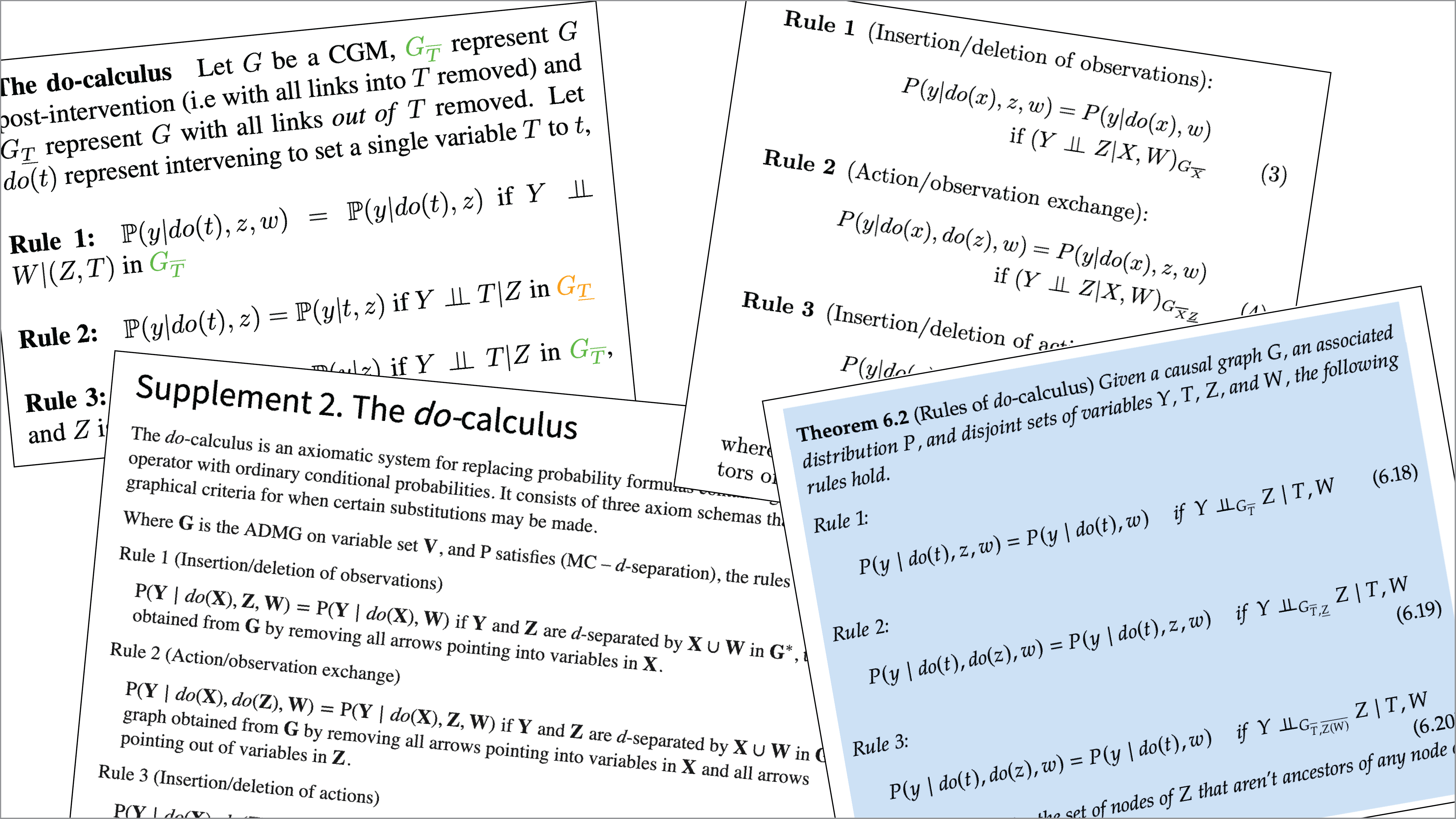
I’ve been teaching a course on program evaluation since Fall 2019, and while part of the class is focused on logic models and the more managerial aspects of evaluation, the bulk of the class is focused on causal inference. Ever since reading Judea Pearl’s The Book of Why in 2019, I’ve thrown myself into the world of DAGs, econometrics, and general causal inference, and I’ve been both teaching it and using it in research ever since.
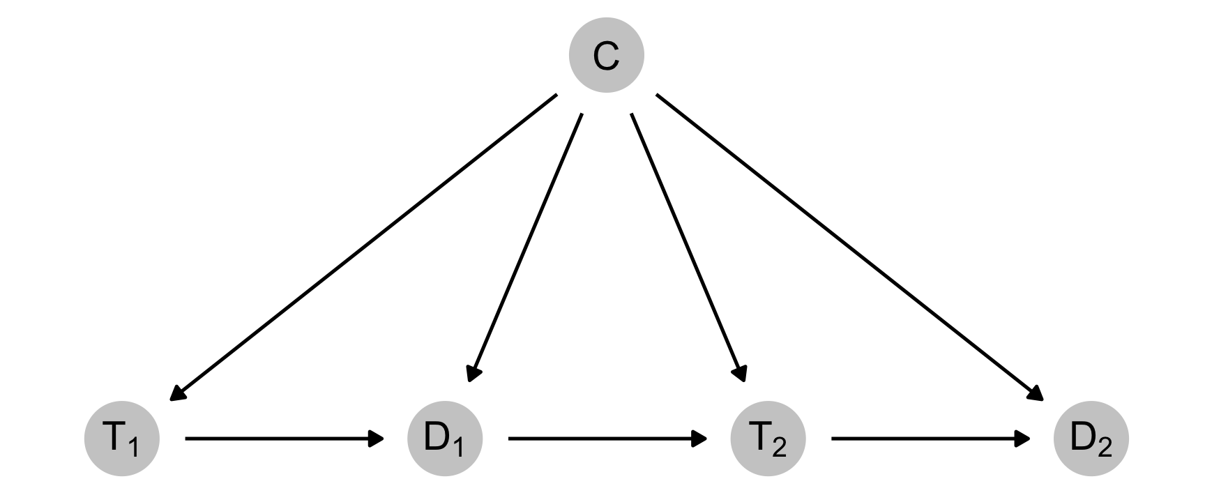
Since my last two blog posts on binary and continuous inverse probability weights (IPWs) and marginal structural models (MSMs) for time-series cross-sectional (TSCS) panel data, I’ve spent a ton of time trying to figure out why I couldn’t recover the exact causal effect I had built in to those examples when using panel data. It was a mystery, and it took weeks to figure out what was happening.

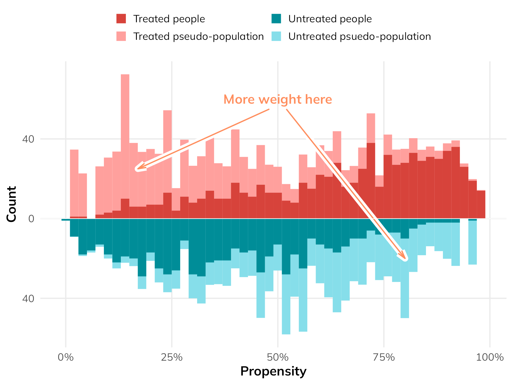
In my post on generating inverse probability weights for both binary and continuous treatments, I mentioned that I’d eventually need to figure out how to deal with more complex data structures and causal models where treatments, outcomes, and confounders vary over time.
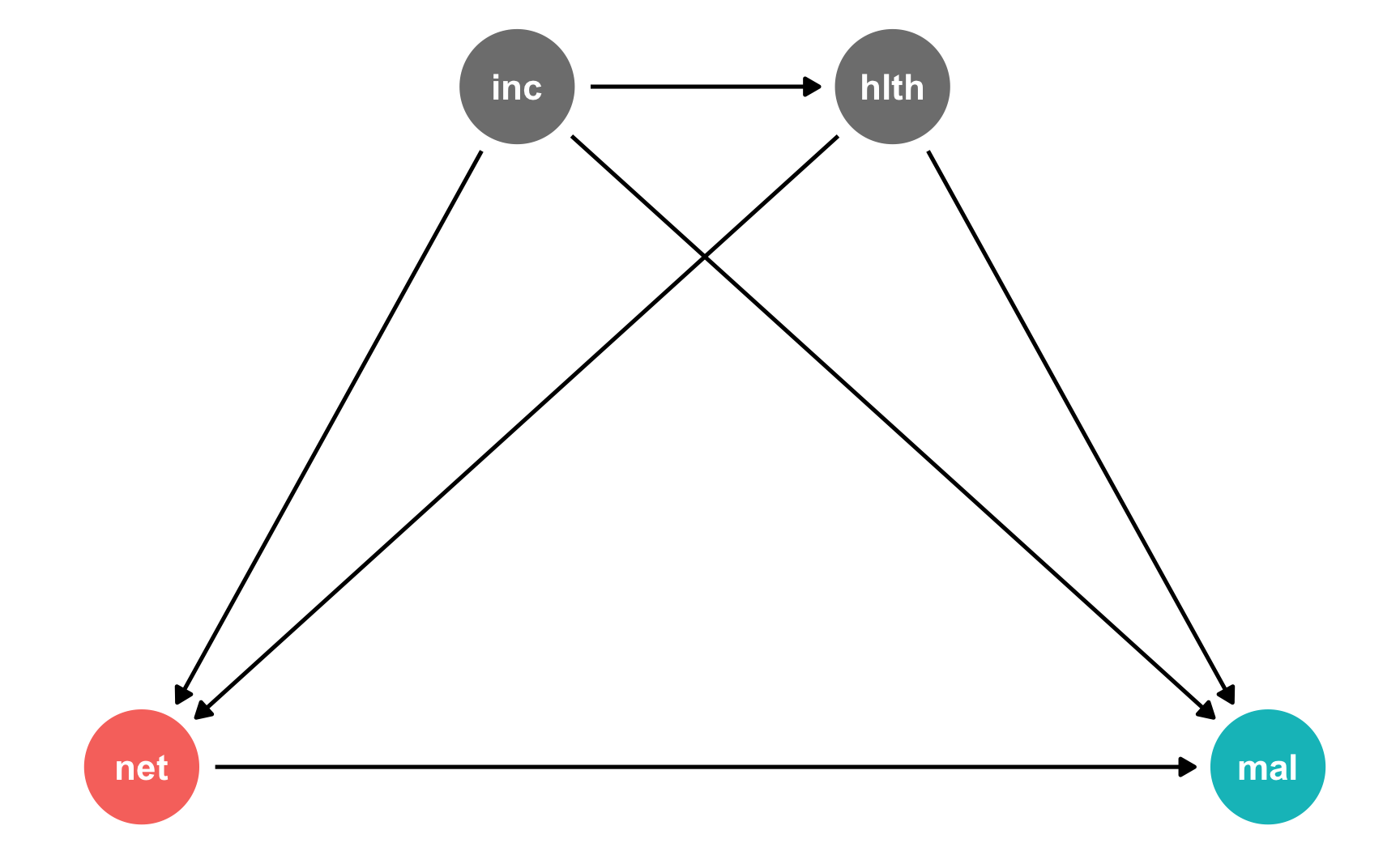
My program evaluation class is basically a fun wrapper around topics in causal inference and econometrics. I’m a big fan of Judea Pearl-style “causal revolution” causal graphs (or DAGs), and they’ve made it easier for both me and my students to understand econometric approaches like diff-in-diff, regression discontinuity, and instrumental variables.